Menu
Recently, a coworker asked me about a query performance problem that had suddenly arisen as they so often do. During testing, this particular query had performed extremely quickly, but when it was shown to a C-level person, it dragged terribly making this impatient person wait 80 seconds for the answer to come back. We all know how valuable their time is, so this had to be solved quickly. He showed me the query, which I had never seen before, along with the execution plan. An execution plan comprises the steps by which SQL Server provides the answer to a query and SSMS provides graphical representations of this mechanism. The graphical plans take two forms: estimated and actual. An estimated plan is what SQL Server anticipates it will do, whereas an actual plan shows what it really did. Database statistics and other factors, e.g., the number of indices, may create significant differences between the two. If possible, the actual plan is the better choice, but sometimes the problematic query runs too long or cannot be executed in the current environment because it changes the database and the locking may create bottlenecks. In these cases, the estimated plan must suffice.
Since the execution plan provides a complete picture of how SQL Server did things (assuming an actual plan), knowing how to interpret these plans is critical for solving performance problems as quickly as possible. In the aforementioned case, the analysis, discussion, and experimentation process only required about 45 minutes to reduce the execution time from 80 seconds to 3 seconds. It also helped everyone understand the data better so these kinds of issues will be less likely to occur in the future.
When a query contains multiple statements, multiple query execution plans are drawn. Nodes, i.e., operators, comprise an execution plan that is also known as a query plan. These nodes specify the operation that will be performed as part of the query or statement. Each node is connected to a parent node by arrows that indicate the estimated or actual number of rows produced by the operator. As shown in Figure 1 and Figure 2 below, the width of the arrow is proportional to the number of rows returned, e.g., an operator that returns 5.5 million rows will be extremely wide whereas one that returns one hundred rows will be very thin.
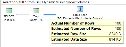
Figure 1: Arrow Thickness Example – Small Number of Rows
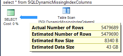
Figure 2: Arrow Thickness Example – Large Number of Rows
Details concerning a particular operator can be obtained by hovering over the operator as shown in Figure 3. For complete details, shown in Figure 4, select the operator, right click, and select properties.
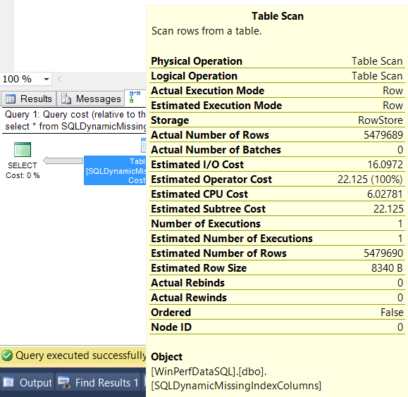
Figure 3: Operator Details Popup
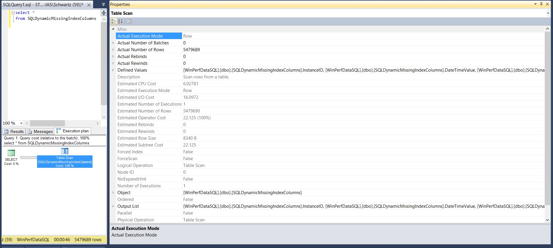
Figure 4: Operator Details Properties Pane
The plan below illustrates a simple and efficient execution plan. The SQLTraceReceiver Table contained 20,815,160 rows and the query returned only 243. Only 979 logical reads were performed, the CPU time was 16 milliseconds, and the duration was 2,194 milliseconds (or 2.194 seconds). As cited previously, the arrow widths are very thin indicating that the smallest amount of data possible was returned. This is supported by the fact that a NonClustered Index Seek operator, which looks up a row in the NonClustered index using a key, was used against the ix_AppName index. The Key Lookup operator obtains data from the underlying clustered index. In this particular case, the * in the output list of the select statement causes the Key Lookup. To summarize, SQL Server uses the ix_AppName index to navigate to a specific record and then returns all the columns of that record using the Key Lookup operator.
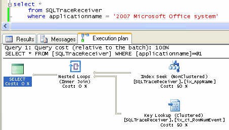
Figure 5: Efficient Execution Plan
The plan below illustrates an inefficient execution plan. In this case, the use of the ISNULL function in the where clause forces SQL Server to rummage through ALL of the 20+ million records in the table to find the desired 243. A Clustered Index Scan does exactly what its name suggests: it scans the entire table, which in this case, is a clustered index. It is important to note the little arrows in the beige circle. This indicates a parallelized operator and means that the problem is so large it must be broken up into MAXDOP pieces to complete in as timely a manner as possible. Whenever you see a plan with scans of large tables and parallel operator indicators, the query is most likely going to perform poorly. Note: small tables will be scanned regardless, so it is important to understand the number of rows in a table before jumping to the conclusion that the scan is necessarily bad. Although this plan looks simpler, it is much worse in terms of performance as indicated by the following statistics:
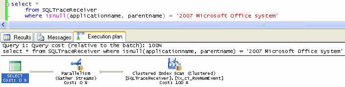
Figure 6: Inefficient Execution Plan
The following table summarizes the differences between the two queries: 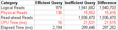
Table 1: Comparison of Efficient and Inefficient Execution Plans
Clearly, the first plan was far more efficient and both returned the same data.
Understanding execution plans is critically important for analysts because they enable them to understand why a query that usually runs perfectly, suddenly and consistently takes forever with different parameters. Although this article only discusses a few operators, they are some of the most important ones to examine when a query performs poorly.